Turbulent Flow PINN

Crafted by Bob Bu · Winter 2024

Traditional Computational fluid dynamics simulation is often bottlenecked by tiny time steps imposed by Courant limits. Simulations can range from tens of core-hours for simple cases to billions for NASA's high-fidelity turbulence studies. This raises a fundamental question: while we gain accurate physical modeling, are we sacrificing too much in terms of runtime, especially for applications like real-time water or air effects in video games?

With the rise of neural networks, a new approach called Physics-Informed Neural Networks (PINNs) brings that question to everyone's desk. This project explores and validates that trade-off and shows it's possible to balance physical accuracy with interactivity and real-time visualization.

This clip provides the ground-truth flow field used to train the neural network model. It depicts a Boeing 737 MAX 8 twin-engine narrow-body on approach with flaps 20, landing gear extended, and an airspeed of 130 knots, typical final approach configuration for this aircraft.

The scene was later solved using a k-omega-SST Improved Delayed Detached Eddy Simulation (kOmegaSSTIDDES) model, and the raw data were post-processed in ParaView to generate the Q-criterion surfaces and colored streamlines shown in the video.

OpenFOAM, an open-source CFD solver, was chosen to generate high-fidelity fluid simulation data. This data was then used to train a Physics-Informed Neural Network (PINN), which I validated in a controlled test scenario with real-time visualization. The model reconstructs turbulent flow behavior in a Tesla valve using a deep neural network guided by physical laws. It supports real-time output streaming and allows interactive control over flow direction switching.

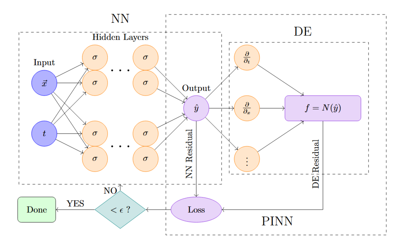
Think of a Physics-Informed Neural Network as two modules stitched together. The first is a standard feed-forward neural network: it takes in space-time coordinates, processes them through multiple hidden layers, and outputs a prediction for the flow variables. Right beside it is a physics layer. Using automatic differentiation, we can compute all the partial derivatives required by the governing equations.

These derivatives are directly inserted into the Navier-Stokes and turbulence equations, producing residuals that measure how much the prediction violates physical laws. The data loss (how far the prediction is from any known data) and the physics loss (how far it breaks the equations) are combined. Gradient descent minimizes this total loss. Once the model fits both the data and the physics to a satisfactory level, training is complete.

def physics_loss(model, inputs, rho=1.225, mu=1.8375e-5, beta=0.075, ...):
    inputs.requires_grad_(True)
    u, v, w, k, omega, p = model(inputs).T

    # Helper for ∂/∂x, ∂/∂y, ∂/∂z, ∂/∂t
    def grad_f(y):
        return torch.autograd.grad(
            y, inputs, torch.ones_like(y),
            create_graph=True, retain_graph=True
        )[0]

    du = grad_f(u)
    dv = grad_f(v)
    dw = grad_f(w)
    dk = grad_f(k)
    domega = grad_f(omega)
    dp = grad_f(p)

    # Continuity: ∇·u = 0
    continuity_res = du[:, 0] + dv[:, 1] + dw[:, 2]

    # Momentum: ρ Du/Dt = −∇p + μ∇²u
    lap_u = grad_f(du[:, 0])[:, 0] + grad_f(du[:, 0])[:, 1] + grad_f(du[:, 0])[:, 2]
    momentum_x_res = (
        du[:, 3] + u * du[:, 0] + v * du[:, 1] + w * du[:, 2]
        + (1.0 / ρ) * dp[:, 0]
        - (μ / ρ) * lap_u
    )
    # y- and z-components built the same way

    # Turbulence: SST k-ω model
    P_k = (k / (omega + 1e-12)) * (du**2 + dv**2 + dw**2).sum(dim=1)
    lap_k = grad_f(dk[:, 0]).sum(dim=1)
    k_res = (
        dk[:, 3] + u * dk[:, 0] + v * dk[:, 1] + w * dk[:, 2]
        - P_k + β * ρ * k * omega
        - (μ / ρ) * lap_k
    )
    # ω-equation analogous

    return (
        (continuity_res**2).mean()
        + (momentum_x_res**2).mean()
        + (k_res**2).mean()
        + ... # Final physics penalty
    )

This function builds the physics-based loss for training a PINN. Using PyTorch's autograd, it calculates spatial and time derivatives directly from the model's output. It enforces six partial differential equations: continuity, momentum in three directions, and two turbulence transport equations.

The Navier-Stokes equations describe the motion of fluid substances by capturing the balance of physical quantities. The continuity equation ensures mass conservation, while the momentum equations enforce momentum conservation under the influences of pressure, viscosity, and inertia.

Each is converted into a mean-square residual. Turbulence effects are modeled via an eddy-viscosity term computed from the predicted energy and dissipation rate. The final loss combines all residuals into a single scalar for neural network optimization.

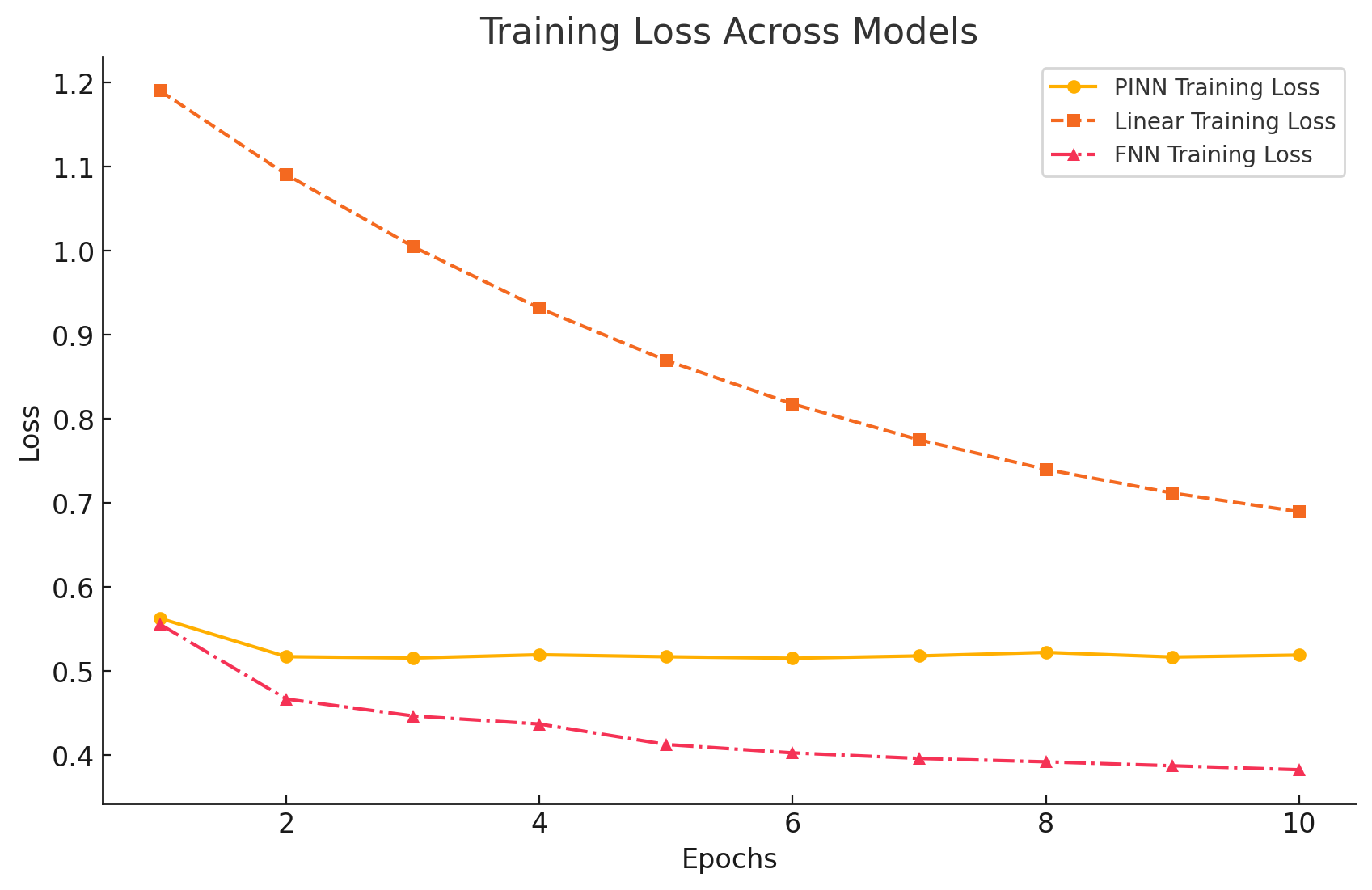
Across ten training epochs on a dataset of approximately twenty million points (10M points for training, 10M for validation, batch size 4096), the three models drift in different directions. The linear fit slashes its training loss the quickest, the plain FNN follows, and the PINN, which carries that extra physics penalty, levels off a little higher.

Flip to the validation curve, though, and the picture tilts. After the first couple of epochs, the PINN edges ahead and keeps the lowest error, while the other two trail just behind. In other words, the physics term costs a bit in-sample but will pay back once the model steps outside the data it saw during training.

In the validation test scene, a Tesla valve geometry is loaded as a single STL mesh. At each time step, field values are streamed directly from the trained PINN, allowing the viewer to update in real time with smooth performance across both macOS and Windows platforms.

Under reverse flow, pressure contours shift from red to blue as mild recirculation develops within the loops. Flow separation becomes visible, and the stream weakens progressively, showing increased resistance compared to the forward case.

When the direction is switched, the same path produces a smoother pressure gradient and a more focused stream with minimal disruption, indicating that the valve geometry supports asymmetric flow behavior as originally intended by the Serbian-American engineer Nikola Tesla:

The interior of the conduit is provided with enlargements, recesses, projections, baffles, or buckets which, while offering virtually no resistance to the passage of the fluid in one direction, other than surface friction, constitute an almost impassable barrier to its flow in the opposite direction.

You can download the files from GitHub and run the demo scene by executing 'TeslaValveFlowSimulator.py' in Python. It will load the geometry and use a pre-trained neural network to predict and visualize the flow in real time. If you’d like to generate your own CFD data, the OpenFOAM configuration files and 3D geometry models are also provided.

University of Alberta · Edmonton, AB, Canada