Optical Flow Tracker
Crafted by Bob Bu · Spring 2025
This is an OpenCV project that tracks feature points in video using optical flow for motion visualization and computer vision tracking. The gradient-based pipeline first compute temporal and spatial derivatives, then solve for the flow vector over a window or over patches.


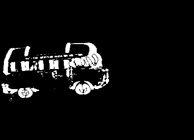
For two consecutive grayscale frames and , the temporal gradient is computed as the frame difference
A threshold on helps isolate motion-dominant changes and suppress low-amplitude noise before solving for motion.
Spatial gradients are computed using forward differences along the horizontal and vertical axes
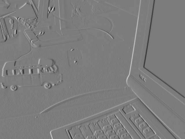
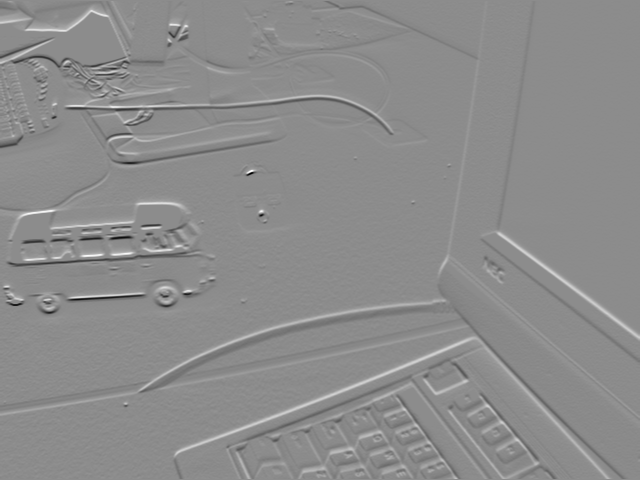
With , , and , the optical flow constraint is written as
Solving this relation within a selected region yields a motion vector field.
Single-window flow assumes motion is approximately uniform inside the window, which can fail when multiple objects move differently or when motion contains rotation or scale changes.
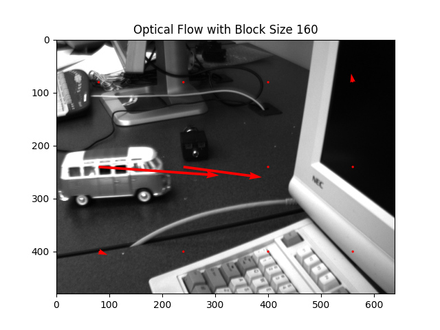
To improve stability, the image can be divided into non-overlapping patches of size . A single flow vector is solved per patch, representing average motion within that region. Increasing reduces noise by averaging over a larger area, while decreasing it preserves finer motion detail.
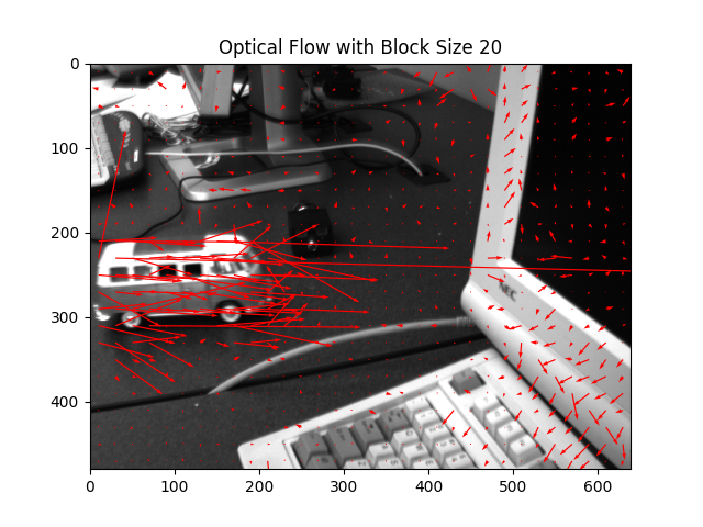


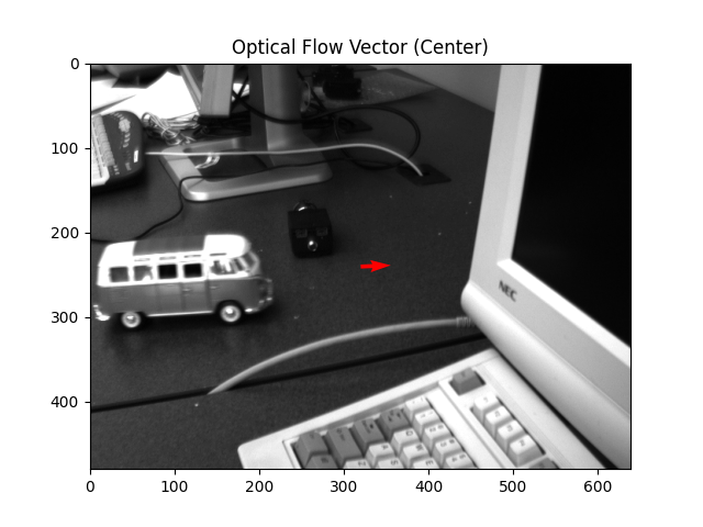
For a given video, the tracker runs frame-by-frame and renders motion vectors on top of the video. Optical flow works best when brightness is approximately constant, motion between frames is small, and nearby pixels share similar motion.
A good example is when the motion is smooth and small between consecutive frames. Brightness constancy holds as the video has consistent lighting. The scene contains smooth spatial changes.
A bad example violates the small motion assumption: Rapid movements lead to inaccurate vectors. Brightness constancy is violated due to changing lighting or shadows. Complex scenes with multiple overlapping motions violate the spatial smoothness assumption.
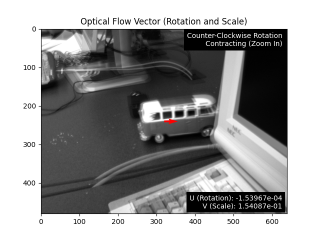
Beyond translation, this project also explores rotation and zoom using gradients tailored to angular and scale change, then solves an optical-flow-like constraint for rotation and scale .
The derivation relies on a first-order Taylor expansion, assuming higher-order terms are negligible under small motion. A common linearization is
When motion is large or intensity changes abruptly, higher-order terms become non-negligible and the linear approximation degrades.
University of Alberta · Edmonton, AB, Canada