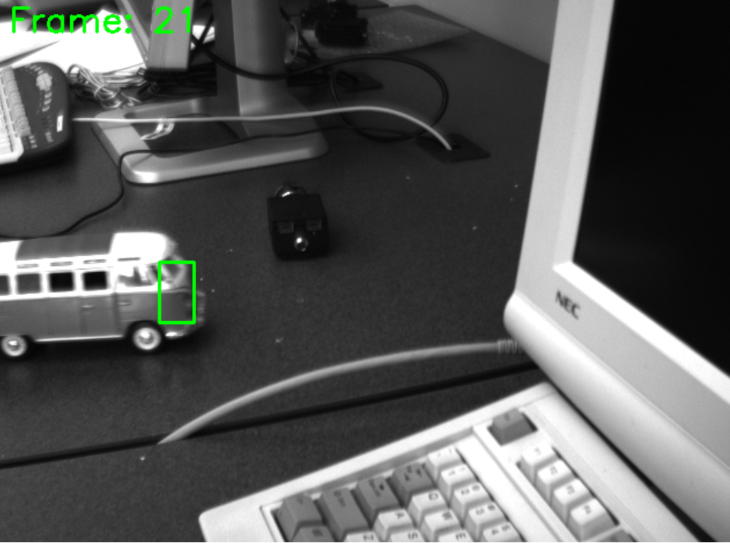
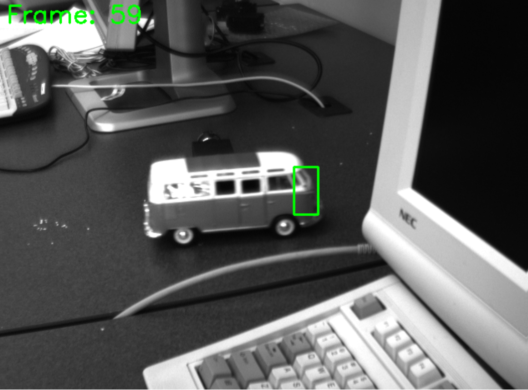
This project implements a Sum of Squared Differences (SSD) tracker for live video. A user-selected ROI is used as the initial template, and the tracker iteratively solves for the displacement vector u=[u,v]T to minimize alignment error across frames.
The ROI is selected on the first frame using cv2.selectROI(), then the template is extracted from the initial image. For the next frame, the tracker estimates the displacement
u=[u,v]T
The update is solved iteratively until convergence or until the maximum number of iterations is reached. A practical stopping rule compares consecutive updates:
∥uk−1∥∥uk∥<thresholdork=max_iterations.
After each iteration, the ROI is shifted by u and the updated bounding box is drawn on the subsequent frame. Iterative warping improves accuracy, but a single update may fail when motion is large.
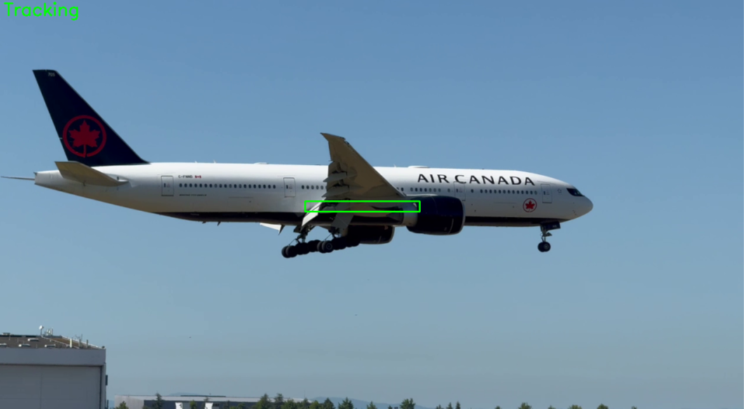
A live tracker processes frames in real time. Two strategies are evaluated and compared in the following airplane scene: keeping a fixed template from the first frame (left picture), and updating the template every frame using the current ROI (right picture). Updating the template adapts to appearance changes (lighting or deformation), but it can also propagate drift when one frame is misaligned.
Applying the tracker to longer sequences shows the typical failure modes. The 2-DoF tracker performs well under smooth motion, consistent lighting, and distinct ROI textures, but it struggles with rapid motion, occlusion, and strong perspective or appearance changes. To handle these cases, higher-DoF warps can model rotation, scale, and projective deformation.
For higher-DoF tracking, a common choice is an 8-DoF homography warp. The mapping from input coordinates (x,y) to output coordinates (u,v) is written in homogeneous form:
uvw=h1h4h7h2h5h8h3h61xy1.
Expanding and normalizing by w gives the projective coordinates:
Warping requires sampling intensity values at subpixel coordinates, so bilinear interpolation is used. Let (u,v) lie within a cell with corner intensities I00,I01,I10,I11 and fractional offsets du and dv:
The optimization follows a Lucas–Kanade / Gauss–Newton derivation. The brightness constancy assumption is
I(W(x;p))=T(x),
and the SSD objective is
E(p)=x∑[T(x)−I(W(x;p))]2.
Linearizing the warped image around p gives
I(W(x;p+Δp))≈I(W(x;p))+∇I(W(x;p))⋅JΔp.
Define the residual e(x)=T(x)−I(W(x;p)). Substituting the approximation yields a linearized least-squares problem and the normal equation
HΔpHb=b,=x∑SD(x)SD(x)T,=x∑SD(x)e(x).
where the steepest descent direction is SD(x)=JT∇I(W(x;p)). For numerical stability, H is factorized using QR decomposition and solved by back-substitution. Parameters update as
p←p+Δp,∥Δp∥<ϵ.
In one controlled test case, the 8-DoF tracker achieved a noticeably lower mean squared error (MSE) than a 6-DoF affine baseline and a non-iterative variant that skips Gauss–Newton refinement.
The gap becomes clearest when the ROI experiences perspective tilt and scale change. The full homography model plus iterative updates keeps the warp locked on, while simpler or non-iterative variants tend to drift over time. Full math derivations and code are available in the GitHub repository.